走向万卡LLM推理集群之路
在迈向“万卡集群”的过程中,笔者遇到了许多问题。Kubernetes 标称支持最多 5000 个节点,这个上限通常是指在默认资源配置下的理论规模,实际中包含大量 Pod、CRD 或复杂控制器等对象时,其可用规模会显著缩水。笔者尚未在开源版本中进行系统性压测,尚不清楚极限配置下的真实能力边界。
然而,在使用 AWS 提供的标准 EKS 服务过程中,笔者发现整体性能瓶颈远低于预期:在仅 60 万 QPM(约合 10k QPS)的请求强度下,apiserver 的缓存已无法同步,resourceVersion 出现严重滞后,更新操作频繁失败,集群进入了不可用状态。这一结果显然与多数人对 Kubernetes 扩展能力的认知存在差距。
因此,笔者逐渐意识到,支撑“万卡”级别的集群不仅需要强大的计算与网络资源,更需要在控制面、组件实现上投入大量工程精力。如果不进行多集群拆分,或对 apiserver 本身进行改造优化,仅依赖 EKS 标准配置,在千卡规模就已遭遇明显瓶颈。
需要说明的是,笔者所参与开发的边端组件远未达到 Kubelet 的成熟水平,控制器实现的性能和健壮性也存在差距。这也进一步暴露出:Kubernetes 本身虽具备高扩展性,但真正支撑万卡规模并非“开箱即用”,而是极其依赖控制面的设计和组件性能的协同演进。
以 AWS EKS 默认配置为例,假设集群包含 1000 节点,要想稳定支撑每个节点 20 QPS 的访问压力,apiserver 已接近饱和极限。Kubelet 作为核心组件,或许能够维持这一负载水平,但自研 controller 若性能不佳,极易拖慢整个集群的反应速度。
如果你的万卡集群全部使用的是 Kubernetes 原生组件,且运行稳定,那么恭喜你,确实享受到了 Kubernetes 高稳定性和高性能带来的红利。
在笔者所参与的系统中,千节点规模下,每个节点的访问频率必须严格控制在 20 QPS 以下,才能保证系统正常运行。这是基于 AWS 提供的标准 apiserver 能力测得的,没有采用如阿里云那样深度改造的控制面架构。
根据笔者了解,阿里云通过限制客户端访问模式、优化 apiserver 架构,确实能稳定支撑到 5000 节点规模。但再往上,势必需要对 apiserver 进一步“动刀”。
因此,对于想要迈向万卡规模的团队,笔者认为可以从两个方向入手:
- 多集群架构:通过拆分集群,缓解单个 apiserver 的压力;
- 组件限流与优化:在标准 Kubernetes 服务中,尽可能减少对 apiserver 的访问频率,控制各组件 QPS,提升控制面稳定性。
无论 Kubernetes 的理论能力多强,如果不控制客户端行为、不优化组件实现,就很难在实际中获得高扩展性的体验。幸运的是,这其中存在大量可以落地的优化空间。
需要重点注意的几点
1. 控制 API Server 的压力
Kubernetes 的 API Server 实际上远没有我们想象中强大。单个节点超过 20 QPS,在 1000 个节点的场景下就会产生 20,000 QPS 的访问量,对 API Server 是非常大的压力,甚至可能导致服务不可用。因此应尽量将单节点的 QPS 控制在 10 以下。
如何控制单节点 QPS
- 避免不必要的失败请求:例如由于
resourceVersion滞后导致的失败,建议使用更严格的 backoff 策略。曾遇到因更新操作使用了get而非直接读 cache,导致失败请求级联增加,一次失败引发一次同步读和同步更新。 - 减少无效更新:Etcd 适合“读多写少”模式,每次调谐应尽量只进行一次更新。确保对象确实发生变更后再发起
update请求,避免“无脑更新”导致无意义的 QPS 激增。当这也是双刃剑,比如在下载任务中,可能下载时间过长没什么正反馈,作用使用者比较难受。 - 使用高层框架:尽量采用如 Kubebuilder 提供的高层封装,避免直接使用
controller-runtime这类底层库。很多开发者对workqueue和informer等机制理解不深,容易写出高 QPS、低质量的控制器逻辑。 - 速度并非越快越好:与 API Server 打交道时,“稳”往往比“快”更重要。大规模节点下不必追求极致速度,否则反而扛不住。
- CRD 设计需注意:在设计 CRD,尤其是
status字段时,应避免定义频繁更新的字段,防止出现“有事没事就更新 status”的情况。 - Informer的DefaultResyncTime可以优先调成1分钟甚至更大,不要使用秒级别的设置。
2. 提升服务稳定性
在大规模节点扩缩容场景下,服务的稳定性至关重要。
节点优雅退出的挑战
- 对于如 LLM 推理任务,优雅退出困难。例如正在流式输出的对象,可能需要几十秒才能完全释放,需在设计上充分考虑。
错误容忍与重试策略
- 快速重试优于指数回退:LLM 服务通常对 SLA 要求较高,例如要提供 1 秒内的 TTFT。使用熔断或指数退避策略可能反而破坏 SLA。建议采用快速、少次数(如 3 次)、跨多个对象的重试机制。
- 容错对象要合理:若当前对象(如某个 vLLM 实例)出现 NCCL 死锁或 runtime error,应立即跳过并选择其他节点,而非对该对象反复重试。
- 流式处理的异常处理:若输出已经过半再出错,需 proxy 缓存已发送内容并判断是否继续。由于采样是非确定性的,重试结果不一致,建议直接 fail fast,不进行中断续传式的重试。
启动速度优化
- 模型下载:
- 使用 P2P 技术(如 Dragonfly)从邻近节点拉取模型文件;
- 借助 CDN 提升模型的下载速度。
- 模型加载:
- 使用内存文件系统效果有限,更直接的做法是预读一遍模型文件至
/dev/null并用vmtouch确保 Page Cache 命中; - 使用更快的 tensor 格式,比如使用一些优化过的序列化与反序列化库。
- 使用内存文件系统效果有限,更直接的做法是预读一遍模型文件至
- 预处理加速:
- 如 CUDA Graph 优化:若硬件和模型固定,可预先缓存 CUDA Graph。但考虑到其占整体启动时间比例较小,该优化优先级较低。
3. 服务发现与健康探测
- 避免依赖 API Server 做服务发现:可以使用配置中心或直接依赖 Kubernetes 的 DNS,如通过 service 的 DNS 解析 pod IP,减少对 API Server 的访问。
- 健康探针的有效性:
- 简单的端口检查不能有效反映 LLM 的运行状态;
- 推荐使用真实业务接口(如
/v1/chat/completion)做健康探测,以及时发现如 vLLM 死锁等问题。
- 异常端点的处理:
- 负载均衡策略问题:如使用 LCF(Least Connection First)策略,异常节点会因连接数少反而被更多请求打中。应通过 Redis 等方式缓存失败节点,临时剔除;
- Cache aware 的调度陷阱:缓存命中率高的节点若已宕机,仍可能承接大量请求,也应类似处理。
4. 监控与告警
- 应关注以下指标:
- SLA:TTFT、TPOT、E2E 时延、吞吐量等;
- Proxy 的调度延迟、负载均衡延迟,这些直接影响 TTFT。
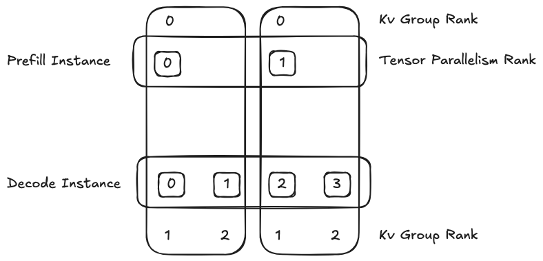
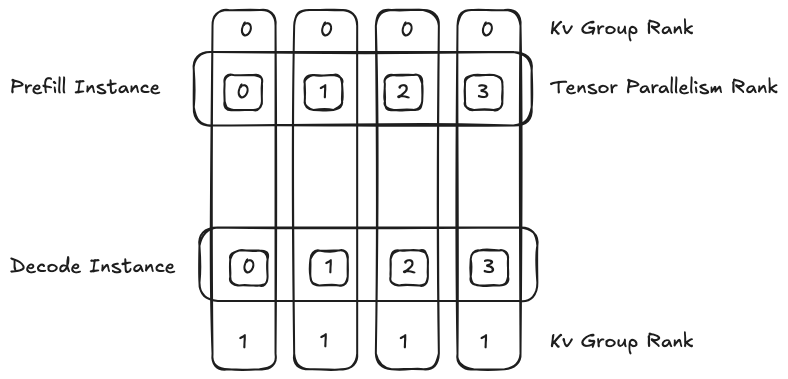
5. PD(Prefill Disaggregation)分离架构
在大规模集群中实现 PD 分离非常具有挑战性,对负载均衡提出更高要求。
- 即便 PD 单独的计算性质比较良好,若在 P2P 场景下负载均衡不佳,整体系统依然会出现性能瓶颈;
- 需设计更精细的分发策略,避免热点节点和数据倾斜。
8. 节点资源异构 & NUMA 绑定
- 问题:大规模集群中,节点配置往往并非完全一致,甚至同一节点上不同 GPU 的性能、带宽、甚至驱动版本都可能略有差异,造成整体推理性能不稳定。
- 优化建议:
- 在资源调度时考虑 GPU 拓扑结构,避免跨 NUMA 节点调度;
- 使用
cudaVisibleDevices精准绑定并确保 GPU memory 布局合理; - 对于 Inference Worker 实现 NUMA-aware 的预绑定机制(如 CPU affinity),可以通过
taskset命令绑定CPU。
- GPU架构的异同:注意管理Nvidia驱动,Cuda版本,高版本一般对低版本是兼容的,笔者经常碰到的问题就是高版本的Cuda无法跑在低版本的驱动上
- 优化建议:
- 保证良好的构建系统,对于编译出的vLLM包能够支持不同GPU的
com_cap版本,像4090是com_cap8.9的,可能生成的代码无法跑在H20的com_cap9.0上。 - 保证机器上的驱动保持在较新的驱动版本,运维要有比较强的更新节奏和意识。
- 如果可以尽量把Cuda装在容器镜像里面,这样可以和宿主机上的Cuda独立,相对来说可以解决一torch版本和cuda版本的不一致的问题,当然这也会导致镜像体积过大,也是一把双刃剑。
- 保证良好的构建系统,对于编译出的vLLM包能够支持不同GPU的
7. 故障演练机制(Chaos Engineering)
- 问题:在万卡规模下,节点、GPU、网络出现异常是常态。没有预演机制会导致“雪崩式”错误放大。
- 优化建议:
- 引入如 Chaos Mesh、Litmus 等框架进行 GPU、网络、文件系统等级别的 fault injection;
- 模拟 API Server 限流、模型加载失败、通信超时、session 丢失等场景;
- 在上线前进行 HA 演练,测试自动恢复和降级路径。
- 准备一些fallover的策略,比如保证一个稳定集群,做集群级别的迁移更新,甚至可以用第三方的供应商去做流量迁移,等升级完成之后再从友商切回来。