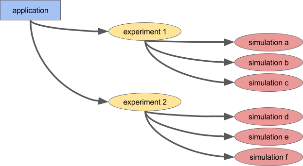
Ray 的基本抽象就是 Remote 或者 Actor,一个是分布式调用函数,一个式分布式调用类。Ray 和 Ray 的 RLlib 主要面对的问题是强化学习有大量的 simulating 的环境,比如仿真一局Dota,涉及到模拟一局Dota,反馈Agent的神经网络,是并行计算和神经网络训练的结合。当然 Ray 本身的抽象就是个分布式 goroutine,所以某种程度上可以完成的事情不光是强化学习一种任务,比如HypterTunning等一些并行计算的模型也是试用的。
反过来想,如果没有 Ray 的话,如何做这个系统呢,要构建大批量的仿真计算环境,然后能根据仿真的反馈训练神经网络。 这两个任务的调度控制就是一个问题,当然放到 k8s 的调度器里做似乎也可以,然后涉及这些分布式任务的同步问题, 需要构建这些任务的关系和信息传输,似乎用一些 DAG (比如 argo)的 workflow 也能解决,但他们之间通信的高效性似乎会是一个问题,需要 选择一种高效的远程调用传输方式,肯能gRPC也可以,还有他们的元数据管理用什么呢,自己搞个Redis似乎也行。 Ray 从这些方面综合考虑了这些问题提供了一个一站式的RL训练平台。
BayesOpt consists of two main components: a Bayesian statistical model for modeling the objective function, and an acquisition function for deciding where to sample next.
Definition: A GP is a (potentially infinte) collection of random variables (RV) such that the joint distribution of every finite subset of RVs is multivariate Gaussian: $ f \sim GP(\mu, k), $ where $\mu(\mathbf{x})$ and $k(\mathbf{x}, \mathbf{x}’)$ are the mean resp. covariance function! Now, in order to model the predictive distribution $P(f_* \mid \mathbf{x}_*, D)$ we can use a Bayesian approach by using a GP prior: $P(f\mid \mathbf{x}) \sim \mathcal{N}(\mu, \Sigma)$ and condition it on the training data $D$ to model the joint distribution of $f=f(X)$ (vector of training observations) and $f_* = f(\mathbf{x}_*)$ (prediction at test input).
采样函数
采样函数一般有 expected improvement(EI),当然还有 probability improvement(PI), upper confidence bound(UCB), knowledge gradient(KG),entropy search and predictive entropy search 等等。 采样的策略有两种: Explore:探索新的点,这种采样有助于估计更准确的; Exploit:利用已有结果附近的点进行采样,从而希望找到更大的;
这两个标准是互相矛盾的,如何在这两者之间寻找一个平衡点可以说是采样函数面对的主要挑战。
Expected improvement is a popular acquisition function owing to its good practical performance and an analytic form that is easy to compute. As the name suggests it rewards evaluation of the objective $f$ based on the expected improvement relative to the current best. If $f^* = \max_i y_i$ is the current best observed outcome and our goal is to maximize $f$, then EI is defined as
The above definition of the EI function assumes that the objective function is observed free of noise. In many types of experiments, such as those found in A/B testing and reinforcement learning, the observations are typically noisy. For these cases, BoTorch implements an efficient variant of EI, called Noisy EI, which allow for optimization of highly noisy outcomes, along with any number of constraints (i.e., ensuring that auxiliary outcomes do not increase or decrease too much). For more on Noisy EI, see our blog post.
Horovod comes with several adjustable “knobs” that can affect runtime performance, including –fusion-threshold-mb and –cycle-time-ms (tensor fusion), –cache-capacity (response cache), and hierarchical collective algorithms –hierarchical-allreduce and –hierarchical-allgather.
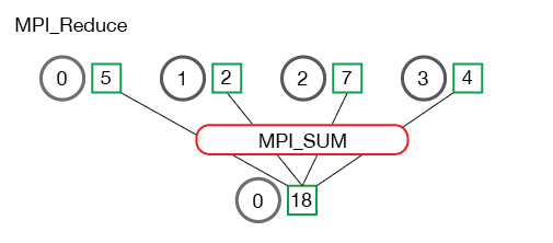
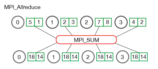
Reduce is a classic concept from functional programming. Data reduction involves reducing a set of numbers into a smaller set of numbers via a function. For example, let’s say we have a list of numbers [1, 2, 3, 4, 5]. Reducing this list of numbers with the sum function would produce sum([1, 2, 3, 4, 5]) = 15. Similarly, the multiplication reduction would yield multiply([1, 2, 3, 4, 5]) = 120.
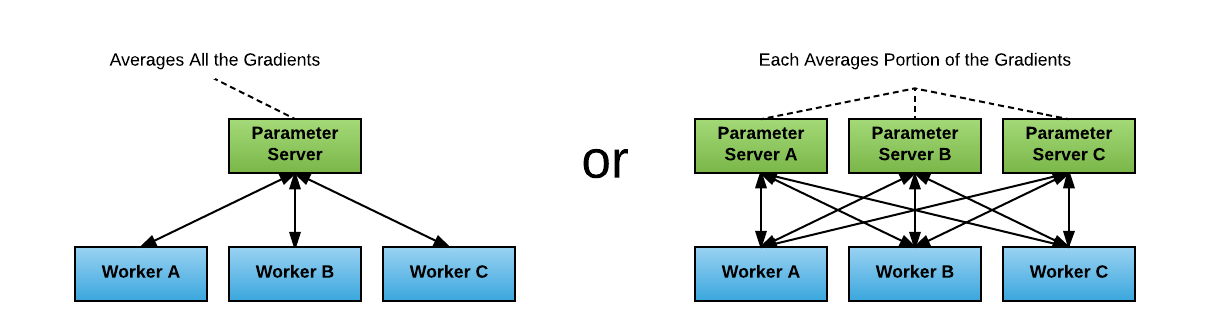
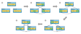
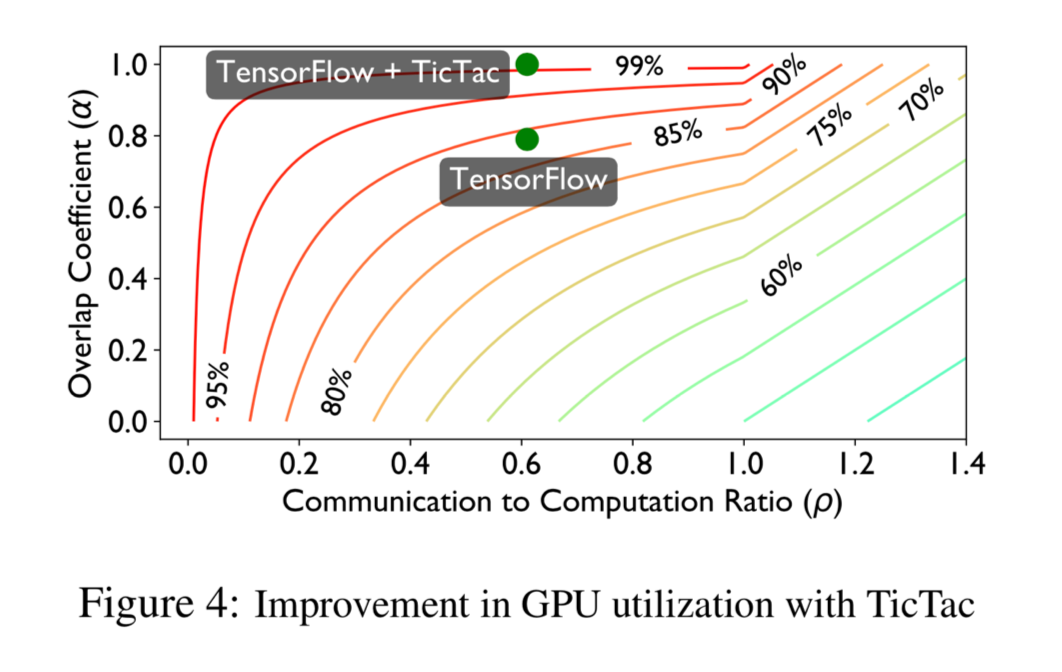
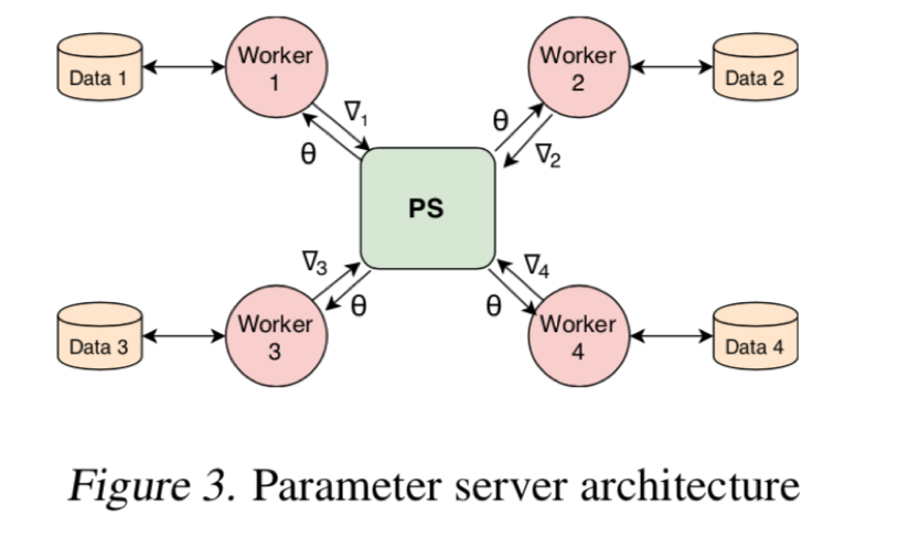
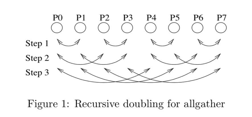
In the system we described, each of the N GPUs will send and receive values N-1 times for the scatter-reduce, and N-1 times for the allgather. Each time, the GPUs will send K / N values, where K is the total number of values in array being summed across the different GPUs. Therefore, the total amount of data transferred to and from every GPU is
Data Transferred=2(N−1)KN
数据传输量在 N 比较大的时候越没有影响,这就消弭了多节点给 Parameter-Server 造成的瓶颈。
第二部根据 local_rank(相当于单节点上的第n张卡),并且设置不占用全部显存,按需分配(可能因内没有统一管理导致显存碎片),然后传递给 keras 设置 session。
1 2 3 4 5
# Horovod: pin GPU to be used to process local rank (one GPU per process)
config = tf.ConfigProto()
config.gpu_options.allow_growth = True
config.gpu_options.visible_device_list = str(hvd.local_rank())
K.set_session(tf.Session(config=config))
# If set > 0, will resume training from a given checkpoint.
resume_from_epoch = 0
for try_epoch in range(args.epochs, 0, -1):
    if os.path.exists(args.checkpoint_format.format(epoch=try_epoch)):
        resume_from_epoch = try_epoch
        break

# Horovod: broadcast resume_from_epoch from rank 0 (which will have
# checkpoints) to other ranks.
resume_from_epoch = hvd.broadcast(resume_from_epoch, 0, name='resume_from_epoch')

# Horovod: print logs on the first worker.
verbose = 1 if hvd.rank() == 0 else 0
# Restore from a previous checkpoint, if initial_epoch is specified. # Horovod: restore on the first worker which will broadcast both model and optimizer weights # to other workers. if resume_from_epoch > 0 and hvd.rank() == 0: model = hvd.load_model(args.checkpoint_format.format(epoch=resume_from_epoch), compression=compression) else: # ResNet-50 model that is included with Keras is optimized for inference. # Add L2 weight decay & adjust BN settings. model_config = model.get_config() for layer, layer_config in zip(model.layers, model_config['layers']): if hasattr(layer, 'kernel_regularizer'): regularizer = keras.regularizers.l2(args.wd) layer_config['config']['kernel_regularizer'] = \ {'class_name': regularizer.__class__.__name__, 'config': regularizer.get_config()} if type(layer) == keras.layers.BatchNormalization: layer_config['config']['momentum'] = 0.9 layer_config['config']['epsilon'] = 1e-5
model = keras.models.Model.from_config(model_config)
# Horovod: adjust learning rate based on number of GPUs. opt = keras.optimizers.SGD(lr=args.base_lr * hvd.size(), momentum=args.momentum)
callbacks = [
    # Horovod: broadcast initial variable states from rank 0 to all other processes.
    # This is necessary to ensure consistent initialization of all workers when
    # training is started with random weights or restored from a checkpoint.
    hvd.callbacks.BroadcastGlobalVariablesCallback(0),

    # Horovod: average metrics among workers at the end of every epoch.
    #
    # Note: This callback must be in the list before the ReduceLROnPlateau,
    # TensorBoard, or other metrics-based callbacks.
    hvd.callbacks.MetricAverageCallback(),

    # Horovod: using `lr = 1.0 * hvd.size()` from the very beginning leads to worse final
    # accuracy. Scale the learning rate `lr = 1.0` ---> `lr = 1.0 * hvd.size()` during
    # the first five epochs. See https://arxiv.org/abs/1706.02677 for details.
    hvd.callbacks.LearningRateWarmupCallback(warmup_epochs=args.warmup_epochs, verbose=verbose),

    # Horovod: after the warmup reduce learning rate by 10 on the 30th, 60th and 80th epochs.
    hvd.callbacks.LearningRateScheduleCallback(start_epoch=args.warmup_epochs, end_epoch=30, multiplier=1.),
    hvd.callbacks.LearningRateScheduleCallback(start_epoch=30, end_epoch=60, multiplier=1e-1),
    hvd.callbacks.LearningRateScheduleCallback(start_epoch=60, end_epoch=80, multiplier=1e-2),
    hvd.callbacks.LearningRateScheduleCallback(start_epoch=80, multiplier=1e-3),
]
最后直接用 allreduce 计算一个 evaluation score。
1
2
# Evaluate the model on the full data set.
score = hvd.allreduce(model.evaluate_generator(input_fn(False, args.train_dir, args.val_batch_size),NUM_IMAGES['validation']))
实现
适配层和压缩算法
horovod 的实现主要分几部分,第一部分是一个适配层,用于兼容各种框架,比如 tensorflow 的适配就是实现一个新的 Op,这个可以参考 add new op,里面规范了 Tensorflow 自定义算子的实现。
请注意,生成的函数将获得一个蛇形名称(以符合 PEP8)。因此,如果您的操作在 C++ 文件中命名为 ZeroOut,则 Python 函数将称为 zero_out。
C++ 的定义是驼峰的,生成出来的 python 函数是下划线小写的,所以最后对应的是,适配Op的代码在 horovod/tensorflow 目录下面
// The coordinator currently follows a master-worker paradigm. Rank zero acts
// as the master (the "coordinator"), whereas all other ranks are simply
// workers. Each rank runs its own background thread which progresses in ticks.
// In each tick, the following actions happen:
//
//      a) The workers send a Request to the coordinator, indicating what
//      they would like to do (which tensor they would like to gather and
//      reduce, as well as their shape and type). They repeat this for every
//      tensor that they would like to operate on.
//
//      b) The workers send an empty "DONE" message to the coordinator to
//      indicate that there are no more tensors they wish to operate on.
//
//      c) The coordinator receives the Requests from the workers, as well
//      as from its own TensorFlow ops, and stores them in a [request table]. The
//      coordinator continues to receive Request messages until it has
//      received MPI_SIZE number of empty "DONE" messages.
//
//      d) The coordinator finds all tensors that are ready to be reduced,
//      gathered, or all operations that result in an error. For each of those,
//      it sends a Response to all the workers. When no more Responses
//      are available, it sends a "DONE" response to the workers. If the process
//      is being shutdown, it instead sends a "SHUTDOWN" response.
//
//      e) The workers listen for Response messages, processing each one by
//      doing the required reduce or gather, until they receive a "DONE"
//      response from the coordinator. At that point, the tick ends.
//      If instead of "DONE" they receive "SHUTDOWN", they exit their background
//      loop.
$$ F=-\frac{G M m r}{(r^2 + \epsilon^2)^{\frac{3}{2}}} $$
这样累加的时候自己也可以加进去,因为 r 是 0,那一项相当于没算。
$$ F_j= \sum_{i=1}^{n} F_i $$
对于 N body 有很多的稍微近似的算法,多是基于实际的物理场景的,比如大部分天体是属于一个星系的,每个星系之间都非常远,所以可以将一些星系作为整体计算,构建一颗树,树中的某些节点是其所有叶子的质心,这样就可以减少计算量,但是放到 GPU 的场景下一个 O(N^2) 的暴力算法利用 GPU 的并行能力可以非常快的算出来。
import math classVector: def__init__(self, x, y, z): self.x = x self.y = y self.z = z def__add__(self, other): return Vector(self.x + other.x, self.y + other.y, self.z + other.z) def__sub__(self, other): return Vector(self.x - other.x, self.y - other.y, self.z - other.z) def__mul__(self, other): return Vector(self.x * other, self.y * other, self.z * other) def__div__(self, other): return Vector(self.x / other, self.y / other, self.z / other) def__eq__(self, other): ifisinstance(other, Vector): returnself.x == other.x andself.y == other.y andself.z == other.z returnFalse def__ne__(self, other): returnnotself.__eq__(other) def__str__(self): return'({x}, {y}, {z})'.format(x=self.x, y=self.y, z=self.z) defabs(self): return math.sqrt(self.x*self.x + self.y*self.y + self.z*self.z) origin = Vector(0, 0, 0) classNBody: def__init__(self, fileName): withopen(fileName, "r") as fh: lines = fh.readlines() gbt = lines[0].split() self.gc = float(gbt[0]) self.bodies = int(gbt[1]) self.timeSteps = int(gbt[2]) self.masses = [0.0for i inrange(self.bodies)] self.positions = [origin for i inrange(self.bodies)] self.velocities = [origin for i inrange(self.bodies)] self.accelerations = [origin for i inrange(self.bodies)] for i inrange(self.bodies): self.masses[i] = float(lines[i*3 + 1]) self.positions[i] = self.__decompose(lines[i*3 + 2]) self.velocities[i] = self.__decompose(lines[i*3 + 3]) print("Contents of", fileName) for line in lines: print(line.rstrip()) print print("Body : x y z |") print(" vx vy vz") def__decompose(self, line): xyz = line.split() x = float(xyz[0]) y = float(xyz[1]) z = float(xyz[2]) return Vector(x, y, z) def__computeAccelerations(self): for i inrange(self.bodies): self.accelerations[i] = origin for j inrange(self.bodies): if i != j: temp = self.gc * self.masses[j] / math.pow((self.positions[i] - self.positions[j]).abs(), 3) self.accelerations[i] += (self.positions[j] - self.positions[i]) * temp returnNone def__computePositions(self): for i inrange(self.bodies): self.positions[i] += self.velocities[i] + self.accelerations[i] * 0.5 returnNone def__computeVelocities(self): for i inrange(self.bodies): self.velocities[i] += self.accelerations[i] returnNone def__resolveCollisions(self): for i inrange(self.bodies): for j inrange(self.bodies): ifself.positions[i] == self.positions[j]: (self.velocities[i], self.velocities[j]) = (self.velocities[j], self.velocities[i]) returnNone defsimulate(self): self.__computeAccelerations() self.__computePositions() self.__computeVelocities() self.__resolveCollisions() returnNone defprintResults(self): fmt = "Body %d : % 8.6f % 8.6f % 8.6f | % 8.6f % 8.6f % 8.6f" for i inrange(self.bodies): print(fmt % (i+1, self.positions[i].x, self.positions[i].y, self.positions[i].z, self.velocities[i].x, self.velocities[i].y, self.velocities[i].z)) returnNone nb = NBody("nbody.txt") for i inrange(nb.timeSteps): print("\nCycle %d" % (i + 1)) nb.simulate() nb.printResults()
CUDA 并行计算
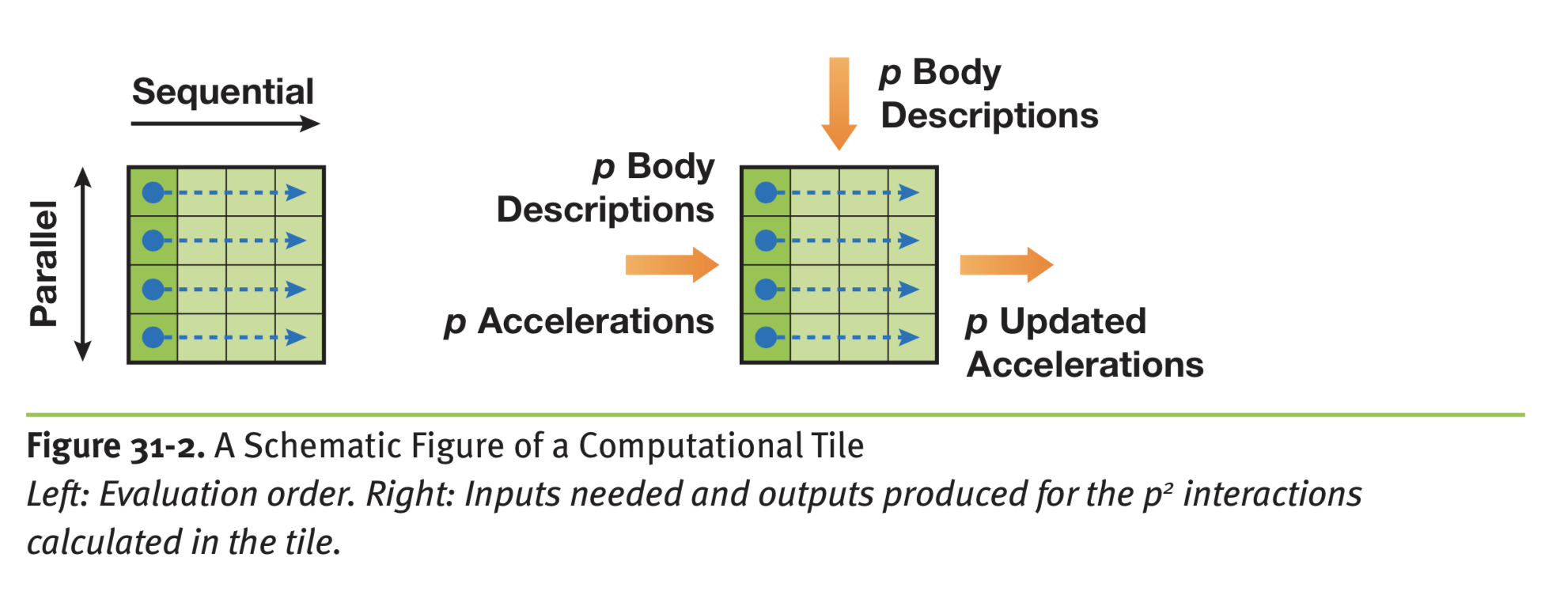
在 CUDA 中并行化首先要理解 CUDA 的层次结构,CUDA 有 grid 和 block 对线程做划分。首先设计一个 computation tile,相当于一个 block 的计算。
左侧表示一个 block 中的 p 个 body 执行 p 次,最后就能更新所有 body 的加速度,这里的内存占用是 O(p) 的不是 O(p^2),浅绿色表示的是串行执行的流,官方的文档没有更新,对应 CUDA 10 的例子里是这样的,vec3 存的是 x/y/z 轴的加速度,vec4 存的是坐标加质量,就是计算 i 受到 j 的加速度,这里没有并行设计是串行的。
第一种用于训练的存档,并且临时恢复,这个时候用户是把训练需要的网络结构在代码里面构造好了的,只是在一定的时间下需要暂时保存网络中的变量,为了在崩溃之后继续训练。所以自然而然会有一个问题,如果我用 Python 写的代码,需要在 C++ 当中恢复,我需要知道你的模型结构,才能恢复,这个最蠢的办法是用 C++ 把你的网络结构再构造一遍,但我们按照统一的协议(比如 Protobuf)确定网络结构,就可以直接从标准序列化的数据中解析网络结构,这就是第二种情况,独立于语言,模型和变量一起保存的情况。然后如果碰到我们不需要再训练了,比如只是把这个模型进行部署,不需要改变相关的变量,那么其实只要一个带常量的模型就可以,这就是第三种情况,把变量冻结的正向传播模型。接下来会依次解释这几种情况的工作方式。
# Add an op to initialize the variables. init_op = tf.global_variables_initializer()
# Add ops to save and restore all the variables. saver = tf.train.Saver()
# Later, launch the model, initialize the variables, do some work, and save the # variables to disk. with tf.Session() as sess: sess.run(init_op) # Do some work with the model. inc_v1.op.run() dec_v2.op.run() # Save the variables to disk. save_path = saver.save(sess, "/tmp/tf-test/model.ckpt") print("Model saved in path: %s" % save_path)
# Add ops to save and restore all the variables. saver = tf.train.Saver()
# Later, launch the model, use the saver to restore variables from disk, and # do some work with the model. with tf.Session() as sess: # Restore variables from disk. saver.restore(sess, "/tmp/tf-test/model.ckpt") print("Model restored.") # Check the values of the variables print("v1 : %s" % v1.eval()) print("v2 : %s" % v2.eval())
MetaGraphDef with tag-set: 'serve' contains the following SignatureDefs:

signature_def['predict_images']:
  The given SavedModel SignatureDef contains the following input(s):
    inputs['images'] tensor_info:
        dtype: DT_FLOAT
        shape: (-1, 784)
        name: x:0
  The given SavedModel SignatureDef contains the following output(s):
    outputs['scores'] tensor_info:
        dtype: DT_FLOAT
        shape: (-1, 10)
        name: y:0
  Method name is: tensorflow/serving/predict

signature_def['serving_default']:
  The given SavedModel SignatureDef contains the following input(s):
    inputs['inputs'] tensor_info:
        dtype: DT_STRING
        shape: unknown_rank
        name: tf_example:0
  The given SavedModel SignatureDef contains the following output(s):
    outputs['classes'] tensor_info:
        dtype: DT_STRING
        shape: (-1, 10)
        name: index_to_string_Lookup:0
    outputs['scores'] tensor_info:
        dtype: DT_FLOAT
        shape: (-1, 10)
        name: TopKV2:0
  Method name is: tensorflow/serving/classify
可以参考 tensorflow 的 REST API,比如 GET http://host:port/v1/models/${MODEL_NAME}[/versions/${MODEL_VERSION}] 其实对应这个例子就是 GET http://host:port/v1/models/tf-test-2/versions/1,然后感觉函数签名不同的 method name,可以调用不同的 request,比如 POST http://host:port/v1/models/${MODEL_NAME}[/versions/${MODEL_VERSION}]:predict 这个格式,如果输入和输出对应的是 images 和 scores 那么就对应了第一个签名。
/** * skb_copy_datagram_iter - Copy a datagram to an iovec iterator. * @skb: buffer to copy * @offset: offset in the buffer to start copying from * @to: iovec iterator to copy to * @len: amount of data to copy from buffer to iovec */ intskb_copy_datagram_iter(conststruct sk_buff *skb, int offset, struct iov_iter *to, int len) { int start = skb_headlen(skb); int i, copy = start - offset, start_off = offset, n; structsk_buff *frag_iter;
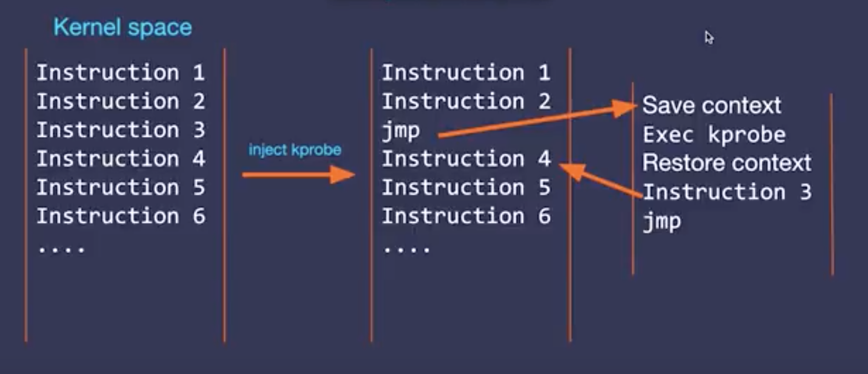
/* skb_copy_datagram_iter() (Kernels >= 3.19) is in charge of copying socket * buffers from kernel to userspace. * * skb_copy_datagram_iter() has an associated tracepoint * (trace_skb_copy_datagram_iovec), which would be more stable than a kprobe but * it lacks the offset argument. */ intkprobe__skb_copy_datagram_iter(struct pt_regs *ctx, conststruct sk_buff *skb, int offset, void *unused_iovec, int len) {
比如判断 method 是不是 DELETE 的是实现就比较蠢,是因为 eBPF 不支持循环,只能这么实现才能把 c 代码翻译成字节码。
// NodeGetId is being deprecated in favor of NodeGetInfo and will be // removed in CSI 1.0. Existing drivers, however, may depend on this // RPC call and hence this RPC call MUST be implemented by the CSI // plugin prior to v1.0. rpc NodeGetId (NodeGetIdRequest) returns (NodeGetIdResponse) { option deprecated = true; }